Invariant and Equivariant Graph Networks

[paper review] : Invariant and Equivariant Graph Networks, ICLR 2019

Motive

Translation Invariance

CNN 의 translation invariant 한 특성은 이미지를 학습하는 데 큰 장점이 됩니다. 이와 같이 translation invariant 한 모델을 만드는 방법으로 Multi-layer perceptron (MLP) 이 있습니다. MLP 를 통해 임의의 연속 함수를 근사할 수 있기 때문에, translation invariant 한 함수 \(f\) 를 모델링하는 MLP 를 만들 수 있습니다. MLP 의 기본적인 형태는 non-linear function \(\sigma\) 와 linear function \(L(x) = Ax+b\) 로 구성된 layer 들로 이루어고, 각 layer 는 \(\mathcal{L}(x) = \sigma(L(x))\) 의 형태를 가집니다.

 

 

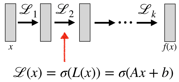
일반적인 MLP 의 경우 input size 가 커질수록, depth 가 깊어질수록 parameter 의 수가 감당할 수 없을 정도로 커집니다. Parameter 의 수를 줄이고 translation invariant 속성을 유지하기 위해서, \(L(x) = Ax+b\) 대신 transform invariant 한 linear operator 를 사용합니다.

 

 

하지만 이미지의 한 픽셀은 다른 임의의 픽셀로 보내지는 translation 을 찾을 수 있기 때문에, transform invariant operator 는 각 픽셀들의 value 를 모두 더해주는 sum operator 와 일치합니다. 모든 픽셀 value 를 더해주는 것은 이미지의 세부 정보를 무시하기에, 의미 있는 operator 라 할 수 없습니다.

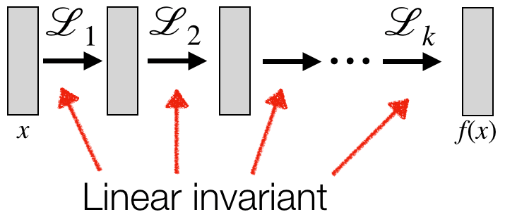
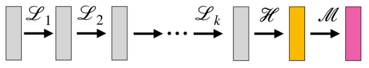
이 때 transform invariant operator 대신, CNN 의 convolution 과 같이 translation equivariant linear operator 를 사용할 수 있습니다. MLP \(m\), invariant linear layer \(h\), non-linear activation \(\sigma\) 와 equivariant linear layer \(L_i\) 들을 통해, 다음과 같이 invariant function \(f\) 를 만들 수 있습니다.

\[f = m\circ h\circ L_k\circ\sigma\circ \cdots \circ\sigma\circ L_1 \tag{1}\]

 

\((1)\) 에서 적절한 layer 들의 선택으로 다양한 invariant model 을 얻을 수 있습니다.

Invariant Graph Networks

이미지에서 translation invariant function 을 통해 feature 를 학습하는 것과 같이, 그래프에서는 permutation invariant function 을 통해 node representation 을 학습할 수 있습니다. 위와 같이 \((1)\) 을 통해 permutation invariant 한 function 을 만들어 낼 수 있고, 이 모델을 Invariant Graph Network (IGN) 라 부릅니다.

 

Graphs as Tensors

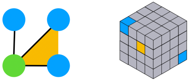
\(n\) 개의 node 를 가진 그래프를 생각해봅시다. 각 node \(i\) 마다 value \(x_i\in\mathbb{R}\) 를 가지고 각 edge \((i,j)\) 마다 value \(x_{ij}\in\mathbb{R}\) 를 가진다면, 이는 \(X\in\mathbb{R}^{n\times n}\) tensor 를 통해 다음과 같이 표현할 수 있습니다.

\[X_{ij} = \begin{cases} x_i &\mbox{ if }\; i=j \\ x_{ij} & \mbox{ if }\; i\neq j \end{cases}\]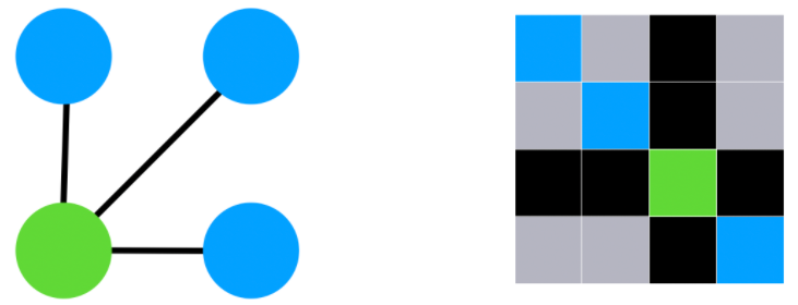

이 표현법을 hypergraph 에 대해서도 일반화할 수 있습니다. \(n\) 개의 node 를 가지는 hypergraph 에 대해, 각 hyper-edge 는 \((i_1,\cdots,i_k)\in [n]^k\) 의 형태로 나타낼 수 있습니다. 따라서 \((1)\) 과 마찬가지로, hypergraph 또한 \(X\in\mathbb{R}^{n^k}\) tensor 로 표현할 수 있습니다.

만약 hyper-edge 들이 \(a\) 차원의 value 를 가진다면, \(X\in\mathbb{R}^{n^k\times a}\) tensor 로 표현할 수 있습니다.

 

Permutation Invariance & Equivariance

이미지에서의 translation 은 symmetry 의 한 종류입니다. 그래프에 있어 symmetry 는 node 순서의 재배열 (re-ordering) 을 통해 해석할 수 있습니다.

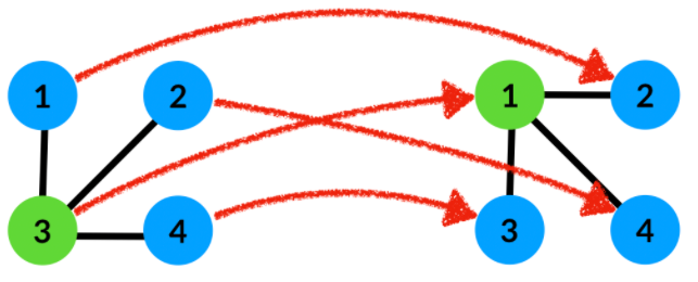
Permutation of Tensors

그래프 node 가 재배열되면, 그에 따라 그래프 tensor 또한 변하게 됩니다.

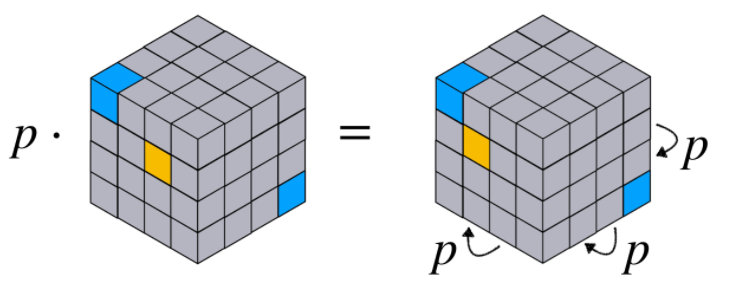
Permutation \(p\in S_n\) 와 \(k\)-tensor \(X\in\mathbb{R}^{n^k}\) 에 대해, \(X\) 에 대한 permutation \(p\) 는 각 hyper-edge \((i_1,\cdots,i_k)\in [n]^k\) 에 대해 다음과 같이 쓸수 있습니다.

\[(p\cdot X)_{i_1,\cdots,i_k} = X_{p^{-1}(i_1),\cdots,p^{-1}(i_k)} \tag{2}\]

Permutation Invariance

함수 \(f\) 가 permutation invariant 하다는 것은, input element 들의 순서와 상관 없이 output 이 같다는 뜻입니다. \(f\) 의 input 이 tensor 일 경우, permutation invariant 는 다음과 같이 나타낼 수 있습니다.

\[f(p\cdot A) = f(A) \tag{3}\]

Permutation Equivariance

함수 \(f\) 가 permutation equivariant 하다는 것은, 임의의 permutation \(p\) 에 대해 \(p\) 와 \(f\) 가 commute 함을 의미합니다. \(f\) 의 input 이 tensor 일 경우, permutation equivariant 는 다음과 같이 나타낼 수 있습니다.

\[f(p\cdot A) = p\cdot f(A) \tag{4}\]

 

Notation

논문에 나오는 notation 들을 정리하면 다음과 같습니다.

notation	explanation
\([\,\cdot\,]\)	\([n]=\{1,\cdots,n\}\)
\(\text{vec}(\,\cdot\,)\)	\(X\) 의 column 들을 쌓아 만든 행렬; \(\mathbb{R}^{a\times b}\) matrix \(X\) 에 대해 \(\text{vec}(X)\in\mathbb{R}^{ab\times 1}\)
\([\text{vec}(\,\cdot\,)]\)	\([\text{vec}(X)]=X\)
\(\otimes\)	Kronecker product
\(P^{\otimes k}\)	\(\overbrace{P\otimes \cdots \otimes P}^{k}\)
\(b(l)\)	\(l\) 번째 bell number

 

Fixed-Point Equations

 

먼저 permutation invariant linear operator 에 대해 알아보겠습니다. 일반적인 linear operator \(L:\mathbb{R}^{n^k}\rightarrow\mathbb{R}\) 을 \(\mathbb{R}^{1\times n^k}\) matrix \(\mathbf{L}\) 로 나타낼 때, \(L\) 이 permutation invaraint 하다면 임의의 permutation \(p\in S_n\) 에 대해 다음을 만족해야합니다.
\(\mathbf{L}\text{vec}(p\cdot A) = \mathbf{L}\text{vec}(A) \tag{5}\)

 

Permutation \(p\in S_n\) 를 나타내는 matrix \(P\) 에 대해 \(\text{vec}(p\cdot A) = P^{T\otimes k}\text{vec}(A)\) 이기 때문에, \((5)\) 는 다음과 같이 쓸 수 있습니다.

\[P^{T\otimes k}\mathbf{L}\text{vec}(A) = \mathbf{L}\text{vec}(A) \tag{6}\]

\((6)\) 은 모든 \(A\in\mathbb{R}^{n^k}\) 에 대해 성립해야하기 때문에,

\[P^{T\otimes k}\mathbf{L} = \mathbf{L} \tag{7}\]

\((7)\) 의 양변에 transpose 를 취하면, 다음의 fixed-point equation 을 얻을 수 있습니다.

\[P^{\otimes k}\text{vec}(\mathbf{L}) = \text{vec}(\mathbf{L}) \tag{8}\]

 

이제 permutation equivariant linear operator 에 대해 알아보겠습니다. 일반적인 linear operator \(L:\mathbb{R}^{n^k}\rightarrow\mathbb{R}^{n^k}\) 을 \(\mathbb{R}^{n^k\times n^k}\) matrix \(\mathbf{L}\) 로 나타낼 때, \(L\) 이 permutaion equivariant 하다면 임의의 permutation \(p\in S_n\) 에 대해 다음을 만족해야합니다.

\[[\mathbf{L}\text{vec}(p\cdot A)] = p\cdot[\mathbf{L}\text{vec}(A)] \tag{9}\]

 

양변에 \(\text{vec}(\cdot)\) 을 취하고 \(\text{vec}(p\cdot A) = P^{T\otimes k}\text{vec}(A)\) 을 이용하면, \((9)\) 를 다음과 같이 쓸 수 있습니다. \(\mathbf{L}P^{T\otimes k}\text{vec}(A) = P^{T\otimes k}\mathbf{L}\text{vec}(A) \tag{10}\)

 

\((10)\) 은 모든 \(A\in\mathbb{R}^{n^k}\) 에 대해 성립해야하며 \(P^{T\otimes k}\) 의 역행렬이 \(P^{\otimes k}\) 이므로, \(P^{\otimes k}\mathbf{L}P^{T\otimes k} = \mathbf{L} \tag{11}\)

 

\((11)\) 의 양변에 \(\text{vec}(\cdot)\) 을 취하고 Kronecker product 의 성질인 \(\text{vec}(XAY) = Y^T\otimes X\text{vec}(A)\) 을 사용하면 다음의 fixed-point equation 을 얻을 수 있습니다. \(P^{\otimes 2k}\text{vec}(\mathbf{L}) = \text{vec}(\mathbf{L}) \tag{12}\)

 

Solving the Fixed-Point Equations

 

모든 permutation invaraint / equivariant 한 linear operator 들을 찾아내는 것은, \((8)\) 과 \((12)\) 의 해를 구하는 것과 같습니다. 즉 다음과 같은 fixed-point equation 의 해 \(X\in\mathbb{R}^{n^l}\) 를 구해야합니다.

\[P^{\otimes l}\text{vec}(X) = \text{vec}(X) \tag{13}\]

 

이 때, \(P^{\otimes l}\text{vec}(X)=\text{vec}(p^{-1}\cdot X)\) 이므로, \((13)\) 은 다음과 같이 정리할 수 있습니다.

\[q\cdot X = X \;\;\text{for all permutation} \;\; q\in S_{n} \tag{14}\]

 

\((14)\) 에 대한 solution space 의 basis 를 특별한 equivalence relation 을 통해 표현하려고 합니다. \(a,\, b\in\mathbb{R}^l\) 에 대해 equivalence relation \(\sim\) 을 다음과 같이 정의하겠습니다.

\[a\sim b \;\text{ iff }\; a_i=a_j \Leftrightarrow b_i=b_j \;\forall i,j\in [\,l\,]\]

\(a\in\mathbb{R}^l\) 에 대해 \(a_i\) 값이 같은 index \(i\) 들로 \([\,l\,]\) 을 분할한 집합을 \(S_a\) 라고 한다면, \(a\sim b\) 임은 \(S_a=S_b\) 와 동치입니다. 따라서, equivalence classes 들은 \([\,l\,]\) 의 분할과 일대일 대응됩니다. 예를 들어, \(l=2\) 라면 equivalence class 는 \(\{a\in\mathbb{R}^2: a_1=a_2\}\) 와 \(\{a\in\mathbb{R}^2: a_1\neq a_2\}\) 두 개 뿐입니다. 이 때 \(\{a\in\mathbb{R}^2: a_1=a_2\}\) 는 \(\{ \{1,2\} \}\) 와, \(\{a\in\mathbb{R}^2: a_1=a_2\}\) 는 \(\{\{1\},\{2\}\}\) 와 대응됩니다. 일대일 대응에 의해, equivalence class 는 총 \(b(l)\) 개 존재합니다.

 

결론적으로, \(X\) 가 \((14)\) 의 해인 것과 \(X\) 가 각각의 equivalence class 내에서 상수라는 것이 동치입니다. 증명은 다음과 같습니다. 먼저 \(X\) 가 각 equivalence class 내에서 상수라고 가정하겠습니다. 임의의 permutation \(q\in S_n\) 와 \(a\mathbb{R}^l\) 에 대해, \(a_i=a_j \Leftrightarrow q(a_i)=q(a_j)\) 이므로 \(a\sim q(a)\) 이고, 가정에 의해 \(X_a=X_{q(a)}\) 를 만족합니다. \((14)\) 에서 양변의 \(a\in\mathbb{R}^l\) 성분을 비교하면 \(X_a=X_{q(a)}\) 이므로, \(X\) 는 \((14)\) 의 해입니다.

반대로, \(X\) 가 \((14)\) 의 해라고 가정하겠습니다. 만약, \(a\sim b\) 라면 permutation \(q\) 가 존재해 \(b=q(a)\) 를 만족합니다. 이 때 \(X_a\neq X_b\) 라면, \(X\) 가 \((14)\) 의 해라는 것에 모순이므로, \(X\) 가 각 equivalence class 내에서 상수여야 합니다.

이제 각 equivalence class \(\gamma\in [n]^l/\sim\) 에 대해 tensor \(B^{\gamma}\in\mathbb{R}^l\) 을 다음과 같이 정의하겠습니다.

\[B^{\gamma}_a = \begin{cases} 1 &\mbox{ if }\; a\in\gamma \\ 0 &\mbox{ otherwise} \end{cases} \tag{15}\]

\((14)\) 의 해 \(X\) 에 대해 \(X\) 가 각 equivalence class 내에서 상수여야 하므로, \(X\) 는 \(B^{\gamma}\) 들의 linear combination 으로 표현할 수 있습니다. 또한 \(B^{\gamma}\) 들의 support 는 disjoint 하므로, orthogonal 합니다. 따라서 \(B^{\gamma}\) 들은 \((14)\) 에 대한 solution space 의 orthogonal basis 를 이룹니다. 이 때, equivalence class 는 총 \(b(l)\) 개 존재하므로 solution space 는 \(b(l)\) 차원입니다.

 

\(n=5\), \(k=2\) 일 때 permutation equivariant linear operator 공간의 orthogonal basis 는 다음과 같습니다.

특히 \(b(2k)=b(4)=15\) 이므로 총 15개의 basis element 가 존재한다는 것을 확인할 수 있습니다.

 

Reference

1. Maron, H., Ben-Hamu, H., Shamir, N., and Lipman, Y. (2019). Invariant and equivariant graph networks. In International Conference on Learning Representations.

2. Zaheer, M., Kottur, S., Ravanbakhsh, S., Poczos, B., Salakhutdinov, R. R., and Smola, A. J. (2017). Deep sets. In Advances in Neural Information Processing Systems, pages 3391–3401.

3. H. Maron, H. Ben-Hamu, H. Serviansky, and Y. Lipman. Provably Powerful Graph Networks. In Neural Information Processing Systems (NeurIPS), pages 2153–2164, 2019.

4. Deep Learning of Irregular Data An Introduction To Invariant Graph Networks (1:2)