Wasserstein Embedding For Graph Learning

[paper review] : WEGL, ICLR 2021

Introduction

 

기존에 graph-structured data 를 분석하는 방식에는 크게 두 가지가 있습니다. 첫 번째는 GNN 을 사용하는 방법입니다. GNN 은 feature aggregation, graph pooling, classification 세 가지를 거쳐 그래프의 representation 을 학습하며, 다양한 domain 에서 좋은 성능을 보여주고 있습니다.

두 번째 방법은 graph kernel 을 이용하는 방법입니다. kernel 을 통해 두 그래프 사이의 similarity 를 표현하여, SVM 과 같은 classifier 를 통해 그래프를 학습합니다. 대표적인 예로 random walk kernel, Weisfeiler-Lehman kernel 등이 있으며, 최근에는 Wasserstein distance 를 활용한 WWL kernel [4] 에 대한 연구가 진행되었습니다.

GNN 과 graph kernel 을 이용하여 그래프를 학습하는 경우, 모두 그래프의 크기가 커질수록 사용하기 힘들어지는 단점이 있습니다. GNN 은 그래프의 크기가 클수록 학습시 필요한 계산량이 많아져 학습이 어려워지며, graph kernel 의 경우 그래프 쌍마다 similarity 를 계산해야하기 때문에 마찬가지로 크기가 큰 그래프 dataset 에 사용하기 어렵습니다.

논문에서는 그래프에 LOT framework [2] 를 적용해 이런 문제를 해결하려고 합니다. GNN 과 graph kernel 의 장점을 모두 사용하기 위해, node embedding 과 LOT framework 를 결합한 Wasserstein Embedding for Graph Learning (WEGL) 를 제시합니다.

 

Background

Wasserstein Distance

\(\mathbb{R}^d\) 에서 정의된 두 probability measure \(\mu\) 와 \(\nu\) 사이의 2-Wasserstein distance 는 다음과 같이 정의합니다 [7].

\[\mathcal{W}_2(\mu,\nu) = \left( \inf_{\pi\in\Pi(\mu,\nu)} \int\Vert x-y\Vert^2_2\,d\pi(x,y) \right)^{1/2} \tag{1}\]

여기서 \(\Pi(\mu,\nu)\) 는 transport plan \(\pi\) 들의 집합으로, 각각의 transport plan \(\pi\) 는 모든 Borel subset \(A\) 와 \(B\) 에 대해 \(\pi(A\times\mathbb{R}^d)=\mu(A)\) 와 \(\pi(\mathbb{R}^d\times B)=\nu(B)\) 를 만족합니다.

특히 \(\mu\) 가 Lebesgue measure 에 대해 absolutely continuous 하다면, Brenier theorem [7, 3] 에 의해 \((1)\) 의 정의는 다음과 동일합니다.

\[\mathcal{W}_2(\mu,\nu) = \left( \inf_{f\in MP(\mu,\nu)} \int \Vert z-f(z)\Vert^2_2\,d\mu(z) \right)^{1/2} \tag{2}\]

여기서 \(MP(\mu,\nu)=\left\{ f:\mathbb{R}^d\rightarrow\mathbb{R}^d \mid \nu(B)=\mu(f^{-1}(B)) \;\; \text{for any Borel set B} \right\}\) 로 정의하며, \(f\in MP(\mu,\nu)\) 를 transport map 이라고 부릅니다. 특히 Brenier theorem [7, 3] 에 의해 optimal transport plan \(\pi^{\ast}\) 는 유일하게 존재하며, \((2)\) 를 만족하는 optimal transport map \(f^{\ast}\) 또한 유일하게 존재합니다. 이를 만족하는 optimal transport map \(f^{\ast}\) 를 Monge map 이라고 부르며, \(T^{\nu}_{\mu}\) 라고 쓰겠습니다.

 

LOT Framework

Linear Optimal Transportation (LOT) framework [2] 는 기존의 optimal transport metric 을 더 빠르게 계산하기 위해 제시된 방법입니다. 기존의 방법은 \(M\) 개의 그래프들에 대해 그래프의 각 쌍마다 2-Wasserstein distance 를 구하려면 총 \(M(M-1)/2\) 번의 거리 계산이 필요하기 때문에, large-scale dataset 에 적용하기 힘듭니다. 이를 해결하기 위해 LOT 는 non-linear 한 distribution space 를 linear 한 function space 로 embedding 시켜, distribution 사이의 복잡한 거리 계산 대신 embedding 사이의 weighted \(L^2\)-norm 을 계산합니다.

 

이를 구체적으로 설명하면 다음과 같습니다. \(\mathbb{R}^n\) 에서 정의되며 bounded second momoent 를 가진 probability measure 들의 집합을 \(\mathcal{P}_2(\mathbb{R}^n)\) 이라고 하겠습니다. 또한 \(\sigma\in\mathcal{P}_2(\mathbb{R}^n)\) 에 대해 다음의 norm 으로 정의된 function space \(L^2(\mathbb{R}^n,\sigma)\) 를 생각하겠습니다.

\[\Vert f\Vert^2_{\sigma} = \int \Vert f(z)\Vert^2_2\,d\sigma(z)\]

Lebesgue measure 에 대해 absolutely continuous 한 measure \(\sigma\in\mathcal{P}_2(\mathbb{R}^n)\) 에 대해, probability measure space 에서 function space 로의 LOT embedding \(F_{\sigma} : \mathcal{P}_2(\mathbb{R}^n) \rightarrow L^2(\mathbb{R}^n,\sigma)\) 를 다음과 같이 정의합니다 [7, 3].

\[F_{\sigma}(\nu) = T^{\nu}_{\sigma} \tag{3}\]

 

Monge map 의 정의에 의해, LOT embedding \(F_{\sigma}\) 는 reference measure \(\sigma\) 로부터의 거리를 보존합니다.

\[\begin{align} \Vert F_{\sigma}(\sigma) - F_{\sigma}(\nu)\Vert_{\sigma} &= \Vert Id-T^{\nu}_{\sigma}\Vert_{\sigma} \\ &= \int \Vert z - T^{\nu}_{\sigma}(z)\Vert^2_2\,d\sigma(z) \\ &= \mathcal{W}_2(\sigma,\nu) \tag{4} \end{align}\]

특히 measure 들 사이의 2-Wasserstein distance 는 LOT embedding 사이의 거리로 근사할 수 있습니다 [7].

\[\mathcal{W}_2(\mu,\nu) \approx \Vert F_{\sigma}(\mu) - F_{\sigma}(\nu)\Vert_{\sigma} \tag{5}\]

 

LOT 는 크게 두 가지 장점이 있습니다. 먼저 measure 들의 거리 계산이 쉬워진다는 것입니다. 두 probability measure 의 2-Wasserstein distance 를 LOT embedding 들의 weighted \(L^2\)-norm \((5)\) 로 근사할 수 있기 때문에, 기존의 방법으로는 \(M\) 개의 그래프에 대해 \(M(M-1)/2\) 개의 LP 를 풀어야했지만, LOT 를 통해 \(M\) 개의 LP 만을 풀면 충분합니다. 또한 LOT embedding 은 linear 하기 때문에, Euclidean structure (e.g. image) 에 적용할 수 있는 PCA 혹은 LDA 와 같은 방법을 사용할 수 있습니다.

 

Linear Wasserstein Embedding

 

기존의 연구들 [4, 5, 8, 9] 과 마찬가지로 논문에서는 그래프 (혹은 그래프의 embedding) 를 하나의 probability distribution 으로 고려합니다. 주어진 그래프들의 embedding \(\left\{ Z_i = \left[ z^i_1,\cdots,z^i_{N_i} \right]^T\in\mathbb{R}^{N_i\times d} \right\}^{M}_{i=1}\) 와 reference embedding \(Z_0 = \left[ z^0_1,\cdots,z^0_{N} \right]^T\in\mathbb{R}^{N\times d}\) 에 대해, 각 embedding 을 다음과 같이 probability measure 로 나타냅니다.

\[\mu_i=\frac{1}{N_i}\sum^{N_j}_{n=1}\delta_{z^i_n}\;,\;\;\mu_0=\frac{1}{N}\sum^N_{l=1}\delta_{z^0_l} \tag{6}\]

이 때 \(\mu_0\) 와 \(\mu_i\) 사이의 optimal transportation plan \(\pi^{\ast}_i\) 은 다음의 LP 를 풀어 얻을 수 있습니다.

\[\pi^{\ast}_{i} = \underset{\pi\in\Pi_i}{\arg\!\min} \sum^{N}_{j=1}\sum^{N_i}_{k=1} \pi_{jk}\Vert z^0_j - z^i_k\Vert^2_2 \tag{7}\] \[\begin{align} \Pi_i = \{ \pi\in\mathbb{R}^{N\times N_i} \;\mid\; &N_i\sum^N_{j=1}\pi_{jk} = N\sum^{N_i}_{k=1}\pi_{jk}=1, \\ &\forall k\in\{1,\cdots,N_i\},\;\forall j\in\{1,\cdots,N\} \} \end{align}\]

 

LOT embedding \((3)\) 을 계산하기 위해서는 \(\mu_0\) 로부터 \(\mu_i\) 로의 Monge map 을 찾아야합니다. 다음과 같이 barycentric projection [2, 7] 을 사용해, \((7)\) 의 optimal transportation plan 으로부터 \(\mu_0\) 에서 \(\mu_i\) 로의 Monge map \(F_i:z^0_j \mapsto \bar{z^0_j}\) 를 근사할 수 있습니다.

\[\bar{z^0_j} = N\sum^{N_i}_{k=1}\pi^{\ast}_{jk}z^i_{k} \tag{8}\]

\((8)\) 을 정리하면 다음과 같이 쓸 수 있습니다.

\[F_i = N\left( \pi^{\ast}_iZ_i \right)\in\mathbb{R}^{N\times d} \tag{9}\]

 

\((3)\) 과 \((9)\) 로부터 \(Z_i\) 의 LOT embedding \(F_{\mu_o}(Z_i)\) 를 다음과 같이 계산할 수 있습니다.

\[F_{\mu_o}(Z_i) = F_i = N\left( \pi^{\ast}_iZ_i \right)\in\mathbb{R}^{N\times d}\]

 

이 때 \(\mu_0\) 와 \(\mu_0\) 사이의 optimal transport plan 은 \(\frac{1}{N}I_{N\times N}\) 이고 \(F_{\mu_o}(Z_0) = Z_0\) 를 만족하므로, reference \(Z_0\) 의 embedding 을 원점으로 설정하기 위해, 각 LOT embedding \(F_{\mu_0}(Z_i)\) 에서 \(Z_0\) 를 빼주는 변환을 생각합니다. 또한 \((5)\) 의 weighted \(L^2\)-norm 계산을 일반적인 \(L^2\)-norm 으로 바꿔주기 위해, LOT embedding 대신 다음의 linear Wasserstein embedding \(\phi(Z_i)\) 를 정의합니다.

\[\phi(Z_i) = (F_i-Z_0)/\sqrt{N}\in\mathbb{R}^{N\times d} \tag{10}\]

 

WEGL : A Linear Wasserstein Embedding for Graphs

 

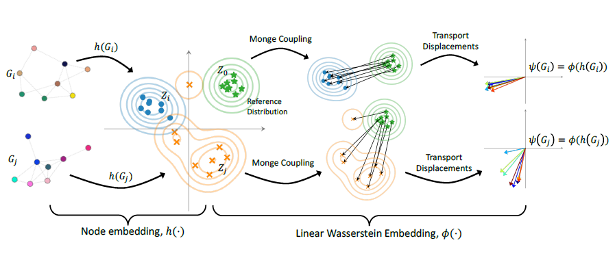
논문에서는 graph classification task 를 위한 Wasserstein Embedding for Graph Learning (WEGL) 를 제시합니다. 먼저 주어진 \(M\) 개의 독립적인 그래프 \(\{G_i=(\mathcal{V}_i,\mathcal{E}_i)\}^{M}_{i=1}\) 들은 diffusion layer 들을 거쳐 node embedding \(\{Z_i\}^{M}_{i=1}\) 로 바뀝니다. 이 후 \(\{Z_i\}^{M}_{i=1}\) 로부터 reference node embedding \(Z_0\) 를 계산하고, \(Z_0\) 에 대한 linear Wasserstein embedding \(\{\phi(Z_i)\}^{M}_{i=1}\) 을 구합니다. 마지막으로, 최종적인 embedding \(\{\phi(Z_i)\}^{M}_{i=1}\) 들을 사용하여 classifier 를 통해 그래프들을 분류됩니다.

WEGL 모델의 input 은 graph dataset, diffusion layer 의 수, final node embedding 의 local pooling 함수, 그리고 classifier 의 종류이며, output 은 그래프의 classification 결과입니다. 다음은 WEGL 의 과정을 표현한 그림입니다.

 

Node embedding

WEGL 의 첫 번째 단계는 그래프들의 node embedding 을 구하는 것입니다. 그래프의 node embedding 에는 다양한 방법이 존재하며 크게 parametric 한 방법과 non-parametric 한 방법으로 나눌 수 있습니다. 만약 parametric embedding 을 사용한다면, 학습 과정에서 node embedding 이 달라질 때마다 linear Wasserstein embedding 을 계산해야합니다. 따라서 WEGL 에서는 복잡한 계산을 줄이기 위해 non-parametric diffusion layer 를 사용합니다.

 

주어진 그래프 \(G=(\mathcal{V},\mathcal{E})\) 의 node feature \(\{x_v\}_{v\in\mathcal{V}}\) 들과 scalar edge feature \(\{w_{uv}\}_{(u,v)\in\mathcal{E}}\) 에 대해, diffusion layer 는 다음과 같이 정의됩니다.

\[x^{(l)}_v = \sum_{u\in N(v)\cup\{v\}}\frac{w_{uv}}{\sqrt{\text{deg}(u)\text{deg}(v)}}\,x^{(l-1)}_u \tag{11}\]

Self-loop \((v,v)\) 를 포함해 scalar edge feature 가 주어지지 않은 edge \((u,v)\) 들에 대해서는 모두 1 로 설정해줍니다. 특히 \((11)\) 에서 \(\sqrt{\text{deg}(u)\text{deg}(v)}\) 를 통해 noramlize 해주는 방법은 GCN 의 propagation rule 에서도 볼 수 있습니다.

 

만약 edge feature 가 scalar 가 아닌 multiple features \(w_{uv}\in\mathbb{R}^{F}\) 로 주어진다면, \((11)\) 의 diffusion layer 를 다음과 같이 바꿔줍니다. 여기서 \(\text{deg}_f(u) = \sum_{v\in\mathcal{V}}w_{uv,f}\) 로 정의합니다.

\[x^{(l)}_v = \sum_{u\in N(v)\cup\{v\}}\left( \sum^F_{f=1}\frac{w_{uv,f}}{\sqrt{\text{deg}_f(u)\text{deg}_f(v)}}\right)\,x^{(l-1)}_u \tag{12}\]

 

마지막으로 node feature \(\{x^{(l)}_v\}^{L}_{l=0}\) 들에 대한 local pooling \(g\) 로 최종 node embedding 을 구합니다.

\[z_v = g\left( \left\{x^{(l)}_v\right\}^{L}_{l=0} \right) \in\mathbb{R}^d \tag{13}\]

\((13)\) 의 local pooling \(g\) 로는 concatenation 또는 averaging 을 사용합니다.

주어진 \(M\) 개의 그래프 \(\left\{G_i=(\mathcal{V}_i,\mathcal{E}_i)\right\}^M_{i=1}\) 들에 대해, node embedding \(\left\{Z_i\right\}^M_{i=1}\) 는 위의 과정을 따라 다음과 같이 표현할 수 있습니다.

\[Z_i = h\left(G_i\right) = \begin{bmatrix} z_1,\;\cdots\;,\;z_{\vert \mathcal{V}_i\vert} \end{bmatrix}^T \in \mathbb{R}^{\vert\mathcal{V}_i\vert\times d}\]

 

Reference Distribution

LOT embedding 을 위한 reference embedding 을 정하는 방법에는 여러 가지가 있으며, 논문에서는 그래프들의 node embedding \(\cup^M_{i=1} Z_i\) 에 대해 \(N=\left\lfloor\frac{1}{M}\sum^M_{i=1}N_i \right\rfloor\) 개의 centroid 들을 가지도록 \(k\)-means clustering 을 통해 reference node embedding \(Z_0\) 을 계산합니다.

또한 node embedding \(\{Z_i\}^{M}_{i=1}\) 들에 대한 Wasserstein barycenter, 혹은 normal distribution 으로부터 뽑은 \(N\) 개의 sample 들로도 reference embedding 을 구성할 수 있습니다. 이론적으로 linear Wasserstein embedding 의 결과는 reference 에 따라 달라지지만, 실험적으로 WEGL 의 성능은 reference 에 따라 큰 차이를 보이지 않습니다.

 

Linear Wasserstein Embedding

\((9)\) 와 \((10)\) 를 통해 reference embedding \(Z_0\) 에 대한 linear Wasserstein embedding \(\phi(Z_i)\in\mathbb{R}^{N\times d}\) 를 계산합니다. 이 때 \((9)\) 를 계산하기 위해 총 \(M\) 개의 LP 를 풀어야합니다. 기존의 Wasserstein distance 를 사용한 방법들은 그래프의 쌍마다 LP 를 풀어야하기 때문에 총 \(M(M-1)/2\) 개의 LP 를 풀어야하므로, linear Wasserstein Embedding 을 사용하면 필요한 계산량이 훨씬 줄어듭니다.

 

Classifier

WEGL 의 최종 단계는 linear Wasserstein embedding \(\{\phi(Z_i)\}^{M}_{i=1}\) 을 사용해 classifier 로 그래프들을 분류하는 것입니다. WEGL 의 장점 중 하나는 task 에 맞는 classifier 를 선택할 수 있다는 점입니다. 논문에서는 classifier 로 AuotML, random forest, RBF kernel 을 이용한 SVM 을 사용했습니다.

 

Experimental Evaluation

 

논문에서는 2 가지의 graph classification task 에 대해 WEGL 의 성능을 평가했습니다.

Molecular Property Prediction

첫 번째 task 는 molecular property prediction task 로 ogbg-molhiv dataset 을 사용했습니다. ogbg-molhiv dataset 은 Open Graph Benchmark 의 일부로 dataset 의 각각의 그래프는 분자를 나타냅니다. 그래프의 node 는 원자를, edge 는 원자들 사이의 결합을 표현하며, 이로부터 각각의 분자가 HIV 를 억제하는지에 대해 이진분류하는 것이 목표입니다.

실험의 baseline 모델로는 GCN, GIN, DeeperGCN, HIMP 를 사용했습니다. 또한 특별하게 ogbg-molhiv dataset 에 대해서는 virtual node 를 사용하는 방법이 좋은 성능을 보여주기 때문에, 각 모델들의 virtual node variant 들과도 성능을 비교했습니다. 각 모델의 성능을 ROC-AUC 로 측정한 결과는 다음과 같습니다.

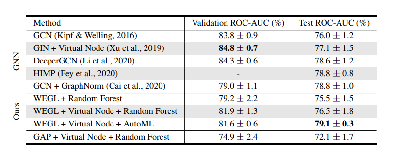
WEGL 에 AutoML classifier 를 사용했을 때 state-of-the-art performance 를 보여주며, random forest classifier 를 사용했을 때도 준수한 성능을 보여줍니다. 특히 GNN 모델들과 같이 end-to-end 학습 없이도 large-scale graph dataset 에 적용될 수 있음을 알 수 있습니다.

또한 linear Wasserstein embedding 의 효과를 입증하기 위한 ablatin study 를 진행했습니다. WEGL 에서 Wasserstein embedding 대신 global average pooling (GAP) 를 사용한 경우 test ROC-AUC 가 확연히 줄어드는 것을 확인할 수 있습니다.

 

TUD Benchmark

두 번째로는 social network, bioinformatics, 그리고 molecular graph dataset 에서 실험을 진행했습니다. 첫 번째 실험과 다르게 GNN baseline 뿐만 아니라, graph classification 에서 좋은 성능을 보여주는 graph kernel 들을 함께 비교했습니다. WEGL 의 classifier 로는 random forest, RBF kernel 을 이용한 SVM, 그리고 GBDT 를 사용했습니다. 각 dataset 들에 대한 graph classification accuracy 는 다음의 표에서 확인할 수 있습니다.

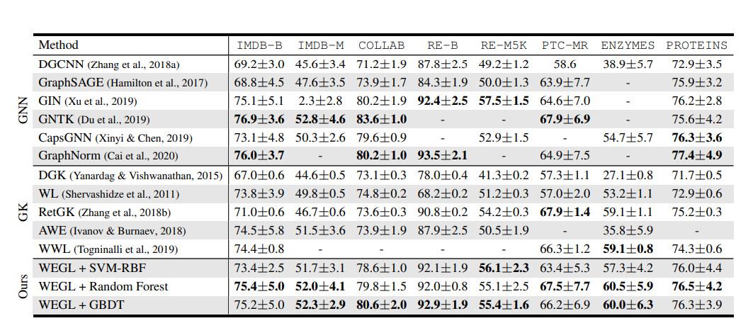
WEGL 은 거의 state-of-the-art performance 에 근접한 성능을 가지는 것을 볼 수 있으며, 특히 모든 dataset 에 대해 top-3 performance 를 보여줍니다. 이로부터 WEGL 이 다양한 domain 에서의 graph 들을 잘 학습함을 알 수 있습니다.

 

Computation Time

마지막으로 WEGL 의 computational efficiency 를 확인하기 위해 학습과 추론에서의 wall-clock time 을 GIN 과 WWL kernel [4] graph kernel 과 비교했습니다. 각 모델의 training time 과 inference time 을 dataset 의 그래프 수, 그래프의 평균적인 node 수, 그리고 그래프의 평균적인 edge 수를 달라히며 측정하였습니다. 결과는 다음의 그래프에서 확인할 수 있습니다.

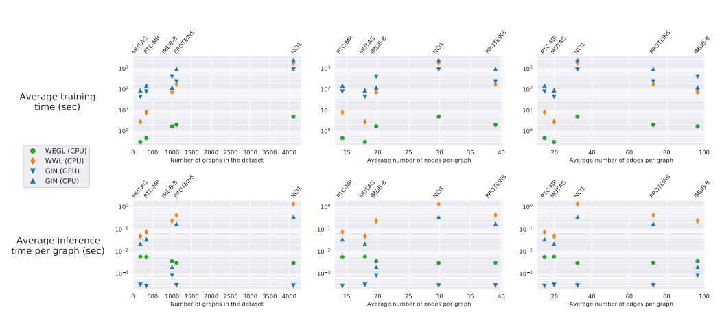
WEGL 은 다른 모델들과 비교해 비슷하거나 훨씬 좋은 성능을 보여줍니다. 특히 그래프의 수가 많아질수록 GIN, WWL 과 비교해 학습 시간이 짧았습니다. GPU 를 사용한 GIN 과 비교해 추론 시간은 조금 길었지만, WEGL 이 CPU 를 사용한 점을 감안하면 그 차이는 크지 않습니다.

 

Future Work

 

WEGL 모델의 단점은 end-to-end 학습이 불가능하다는 것입니다. 특히 GNN 과 같이 node embedding 을 학습하지 않고 non-parametric diffusion layer 를 사용했기 때문에, graph representation 이 제대로 이루어졌는지가 의문입니다. 만약 WEGL 이 end-to-end 학습이 가능하다면, \((6)\) 과 같이 그래프를 probability measure 로 고려할 때, attention 을 적용해 node 마다 다른 weight 을 가지도록 학습하는 방법을 생각해 볼 수 있습니다.

또한 Wasserstein distance (optimal transport) 의 가장 큰 약점은 rescaling, translation, rotation 과 같은 transformation 들에 대해 invariant 하지 못하다는 것입니다. 따라서 Wasserstein distance 대신 Gromov-Wasserstein distance 를 사용한다면, permutation invariant 한 모델을 만들 수 있다고 기대합니다.

마지막으로 \((7)\) 로부터 optimal transport plan 을 계산할 때, entropy regularization 을 적용해 계산을 줄일 수 있습니다. 논문의 실험에서 사용한 dataset 의 크기가 크지 않아 entropy regularization 의 효과가 크지 않았지만, dataset 의 크기가 커질 경우 큰 도움이 될 것입니다.

 

Reference

 

1. Soheil Kolouri, Navid Naderializadeh, Gustavo K Rohde, and Heiko Hoffmann. Wasserstein embedding for graph learning. arXiv preprint arXiv:2006.09430, 2020.

2. Wei Wang, Dejan Slepcev, Saurav Basu, John A Ozolek, and Gustavo K Rohde. A linear optimal transportation framework for quantifying and visualizing variations in sets of images. International Journal of Computer Vision, 101(2):254–269, 2013.

3. Caroline Moosmüller and Alexander Cloninger. Linear optimal transport embedding: Provable fast wasserstein distance computation and classification for nonlinear problems. arXiv preprint arXiv:2008.09165, 2020.

4. Matteo Togninalli, Elisabetta Ghisu, Felipe Llinares-López, Bastian Rieck, and Karsten Borgwardt. Wasserstein Weisfeiler-Lehman graph kernels. In Advances in Neural Information Processing Systems, pp. 6436–6446, 2019.

5. G. Bécigneul, O.-E. Ganea, B. Chen, R. Barzilay, and T. Jaakkola. Optimal Transport Graph Neural Networks. arXiv preprint arXiv:2006.04804

6. WEGL Github code : https://github.com/navid-naderi/WEGL

7. Peyré, G., Cuturi, M., et al. Computational optimal transport. Foundations and Trends® in Machine Learning, 11(5-6):355–607, 2019.

8. T. Vayer, L. Chapel, R. Flamery, R. Tavenard, and N. Courty. Optimal transport for structured data with application on graphs. In International Conference on Machine Learning (ICML), 2019.

9. H. P. Maretic, M. E. Gheche, G. Chierchia, and P. Frossard. GOT: An optimal transport framework for graph comparison. In 33rd Conference on Neural Information Processing Systems (NeurIPS), 2019.