How Powerful are Graph Neural Networks?

[paper review] GIN, ICLR 2019

Related Study

 

GNN 의 expressive power 에 대한 연구는 크게 두 가지 방향으로 이루어집니다. 첫 번째 방법은 이 논문과 같이, Weisfeiler-Lehman (WL) graph isomorphism test 를 통해 GNN 의 expressive power 에 대한 limitation 을 연구합니다 (No. 1, 2, 5). 다른 방향으로는, permutation invariant function 들에 대한 universal approximation 을 통해 GNN 의 expressive power 를 다룹니다 (No. 3, 5). 최근에는 GNN 의 width, depth 와 expressive power 의 연관성에 대한 연구도 이루어졌습니다 (No. 6).

제가 공부하며 expressive power 와 관련된 논문을 아래의 리스트로 정리했습니다.

 

No.	Paper
1	Weisfeiler and Leman Go Neural: Higher-order Graph Neural Networks	Morris et al., 2018
2	Provably Powerful Graph Networks	Maron et al., 2019
3	On the Universality of Invariant Networks	Maron et al., 2019
4	Universal Invariant and Equivariant Graph Neural Networks	Keriven et al., 2019
5	On the equivalence between graph isomorphism testing and function approximation with GNNs	Chen et al., 2019
6	What graph neural networks cannot learn: depth vs width	Loukas, 2020

 

Introduction

 

잘 알려져 있는 Graph Convolutional Network, GraphSAGE, Graph Attention Network, Gated Graph Neural Netowork 등 대부분의 GNN 은 recursive neighborhood aggregation (message passing) scheme 을 사용합니다 [2]. 이런 network 들을 Message Passing Neural Network (MPNN) 이라 부릅니다. MPNN 은 매 iteration 마다 node 주변 neighborhood 의 feature vector (representation) 를 수집하여, node 의 새로운 feature vector 를 update 합니다. \(k\) 번의 iteration 후, 각 node 들은 \(k\)-hop neighborhood 의 feature vector 들로 update 된 새로운 feature vector 를 가지게 됩니다. 충분한 수의 iteration 후에는, 각 node 의 feature vector 가 그래프 전체의 구조에 대한 정보를 포함한다고 해석할 수 있습니다.

Neighborhood aggregataion scheme 을 사용하는 GNN 은 node classification, link prediction, graph classification 등 다양한 task 에 대해 state-of-the-art 성능을 보여줍니다. 하지만, 모델의 설계는 주로 경험적인 직관 혹은 실험을 통한 시행 착오를 통해 이루어집니다. GNN 의 limitation 과 expressive power 등의 이론적인 연구가 바탕이 된다면 더 효율적인 모델을 만들 수 있고, 또한 모델의 hyperparameter tuning 에 큰 도움이 될 것입니다.

논문에서는 GNN 의 expressive power 를 Weisfeiler-Lehman (WL) graph isomorphism test 를 통해 설명합니다. WL test 또한 MPNN 과 같이 매 iteratin 마다 주변 neighborhood 의 feature vector 를 수집해 각 node 의 feature vector 를 update 합니다. WL test 는 regular graph 와 같이 특수한 그래프를 제외하고는, 대부분의 그래프를 구분해낼 수 있습니다 (up to isomorphism). 그 이유는, 바로 알고리즘에서 neighborhood aggregation 이후 node 의 feature vetor 를 update 하는 과정이 injective 하기 때문입니다. WL test 의 알고리즘에서는 그래프의 두 node 가 서로 다른 neighborhood 를 가지고 있다면, 서로 다른 label 을 가지게 됩니다.

Node 의 neighborhood 를 feature vector 들의 multiset 으로 표현하면, GNN 의 neighborhood aggregation scheme 은 multiset 에 대한 함수로 볼 수 있습니다. GNN 이 WL test 와 같이 그래프를 구분할 수 있는 능력 (discriminative power) 이 높지려면, neighborhood aggregation scheme 이 서로 다른 multiset 에 대해 서로다른 embedding 으로 보내주어야 합니다. 따라서, GNN 의 expressive power 를 multiset 에 대한 함수를 통해 분석할 수 있습니다.

 

Preliminaries

 

논문에서 다루는 GNN 들은 모두 MPNN 으로, 매 iteration 마다 각 node 의 neighborhood feature vector 를 수집해 새로운 feature vector 로 update 합니다. 이를 neighborhood aggregation scheme 이라 부르며, 크게 두 단계로 나눌 수 있습니다.

첫번 째 단계에서는, neighborhood 의 feature vector 들을 수집합니다. \(v\) 의 neighborhood \(N(v)\) 에 대해, \(u\in N(v)\) 의 feature vector 들을 모아줍니다. \(k\) 번째 iteration 에서 node \(v\) 의 feature vector 를 \(h_v^{(k)}\) 라고 하면, 다음과 같이 정리할 수 있습니다.

\[a_v^{(k)} = \text{AGGREGATE}^{(k)}\left(\left\{\!\!\left\{h_u^{(k-1)}:u\in N(v)\right\}\!\!\right\}\right)\]

이 때 \(\text{AGGREGATE}\) 함수는 multiset 에 대해 정의된 함수이며, 주로 summation 을 사용합니다. GraphSAGE [4] 에서와 같이 max-pooling 또는 mean-pooling 등을 사용할 수도 있습니다.

두번 째 단계에서는 전 단계에서 수집한 정보 \(a_v^{(k)}\) 와 현재의 feature vector \(h_v^{(k-1)}\) 를 사용해, node 의 새로운 feature vector 를 update 합니다.

\[h_v^{(k)} = \text{COMBINE}^{(k)}\left(h_v^{(k-1)},a_v^{(k)}\right)\]

GraphSAGE 는 vector concatenation \([\,\cdot\,]\) 이후 weight matrix \(W\) 를 이용한 linear mapping 을 통해, 다음과 같은 \(\text{COMBINE}\) 함수를 사용했습니다.

\[\text{COMBINE}^{(k)}\left(h_v^{(k-1)},a_v^{(k)}\right) = W \cdot \left[ h_v^{(k-1)},a_v^{(k)} \right]\]

 

위의 과정을 합치면, MPNN 의 \(k\) 번째 iteration 은 다음과 같이 표현할 수 있습니다.

\[\begin{align} h_v^{(k)} &= \text{COMBINE}^{(k)}\left(h_v^{(k-1)},a_v^{(k)}\right) \\ &= \text{COMBINE}^{(k)}\left(h_v^{(k-1)},\text{AGGREGATE}^{(k)}\left(\left\{\!\!\left\{h_u^{(k-1)}:u\in N(v)\right\}\!\!\right\}\right)\right) \tag{1} \end{align}\]

 

Node classification 에서는 GNN 의 마지막 layer 에서 얻은 feature vector \(h_v^{(K)}\) 들로 prediction 을 수행합니다. Graph classificaiton 의 경우 마지막 layer 에서 얻은 feature vector 들을 모아 \(\text{READOUT}\) 함수를 통해 graph representation \(h_G\) 를 표현하고, 이를 통해 prediction 을 수행합니다.

\[h_G = \text{READOUT}\left( \left\{\!\!\left\{ h_v^{(K)}:v\in V \right\}\!\!\right\} \right) \tag{2}\]

Graph representation \(h_G\) 가 node 의 ordering 에 따라 달라지지 않아야하기 때문에, \(\text{READOUT}\) 함수로 permutation invariant function 을 사용합니다. 간단한 예로 feature 들을 모두 더하는 summation 이 있습니다.

 

Building Powerful Graph Neural Networks

 

WL test 와 GNN 의 representational power 의 관계에 대해 알아보겠습니다.

Weisfeiler-Lehman Test

Lemma 2.

Let \(G_1\) and \(G_2\) be any two non-isomorphic graphs. If a graph neural network \(\mathcal{A}:\mathcal{G}\rightarrow\mathbb{R}^d\) maps \(G_1\) and \(G_2\) to different embeddings, the Weisfeiler-Lehman graph isomorphism test also decides \(G_1\) and \(G_2\) are not isomorphic.

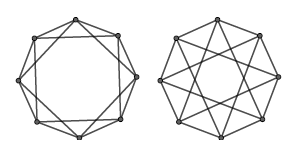
Lemma 2 에 의해, GNN 의 discriminative power 가 WL test 보다 좋을 수 없다는 것을 알 수 있습니다. 즉 WL test 로 구분하지 못하는 그래프들에 대해서는, 예를 들어 다음의 그림과 같이 circular skip link graph 들에 대해서는 GNN 또한 구분할 수 없습니다.

Lemma 2 에 대한 증명의 핵심은 WL test 에서 feature vector 를 update 하는 과정이 injectivite 하다는 것입니다. 그렇다면, 과연 GNN 의 neighborhood aggregation 이 injective 할 때 WL test 와 같은 power 를 가질 수 있을까요? 이에 대한 답은 다음의 Theorem 3 를 통해 얻을 수 있습니다.

Theorem 3.

Let \(\mathcal{A}:\mathcal{G}\rightarrow\mathbb{R}^d\) be a GNN. With a sufficient number of GNN layers, \(\mathcal{A}\) maps any graphs \(G_1\) and \(G_2\) that the Weisfeiler-Lehman test of isomorphism decides as non-isomorphic, to different embeddings if the following conditions hold:

a) \(\mathcal{A}\) aggregates and updates node features iteratively with

\[h_v^{(k)} = \phi\left( h_v^{(k-1)},f\left(\left\{\!\!\left\{ h_u^{(k-1)}:u\in N(v) \right\}\!\!\right\}\right) \right)\]

where the functions \(f\), which operates on multisets, and \(\phi\) are injective.

b) \(\mathcal{A}\) ‘s graph-level readout, which operates on the multiset of node features \(\left\{\!\!\left\{ h_v^{(k)}\right\}\!\!\right\}\), is injective

Theorem 3 에서 함수 \(f\) 와 \(\phi\) 는 각각 위에서 설명한 \(\text{AGGREGATE}\) 와 \(\text{COMBINE}\) 함수에 해당하며, graph-level readout 은 \(\text{READOUT}\) 함수를 의미합니다. 즉 \(\text{AGGREGATE}\), \(\text{COMBINE}\) 과 \(\text{READOUT}\) 이 모두 multiset 에 대해 injective 일때, GNN 은 WL test 와 같은 discriminative power 를 가질 수 있다는 것이 Theorem 3 의 결론입니다.

Lemma 2 와 Theorem 3 에 의해, neighborhood aggregation scheme 을 사용하는 GNN 의 discriminative power 에 대한 upper bound 를 WL test 를 통해 나타낼 수 있습니다.

GNN is at most as powerful as WL test in distinguishing different graphs.

그래프를 구분하는 능력에 있어 GNN 이 WL test 보다 성능이 떨어진다면, GNN 을 쓰는 이유가 무엇인지에 대해 생각해보아야 합니다. GNN 의 가장 큰 장점은 바로 그래프 사이의 similarity 에 대해 학습할 수 있다는 것입니다. WL test 에서의 feature vector 는 label 로 one-hot encoding 에 불과합니다. 두 그래프가 다르다는 것은 확실히 알 수 있어도, 얼마나 다른지에 대해서는 알 수 없습니다. 하지만 GNN 의 feature vector 를 통해 그래프를 구분하는 것 뿐만 아니라, 비슷한 그래프를 비슷한 embedding 으로 보내주도록 학습할 수 있습니다. 즉 두 그래프가 얼마나 다른지에 대해서도 알 수 있습니다. 이런 특성 덕분에, 다양한 분야에서 GNN 이 훌륭한 성과를 보여준다고 생각합니다.

 

Graph Isomorphism Network

 

WL test 와 같은 discriminative power 를 가지는 GNN 을 만들기 위해서는, Theorem 3 에 의해 \((1)\) 의 \(\text{AGGREGATE}\) 와 \(\text{COMBINE}\) 함수가 mutiset 에 대해 injective 해야합니다. 그렇다면, 먼저 multiset 에 대해 injective 한 함수가 존재하는지를 알아야합니다. 다음의 Lemma 5 와 Corollary 6 에서 답을 찾을 수 있습니다. 논문에서는 node 의 input feature space \(\chi\) 가 countable universe 라고 가정합니다.

Lemma 5.

Assume \(\chi\) is countable. There exists a function \(f:\chi \rightarrow\mathbb{R}^n\) so that \(h(X)=\sum_{x\in X}f(x)\) is unique for each multiset \(X\subset\chi\) of bounded size. Moreover, any multiset function \(g\) can be decomposed as \(g(X)=\phi\left(\sum_{x\in X}f(x)\right)\) for some function \(\phi\).

Corollary 6.

Assume \(\chi\) is countable. There exists a function \(f:\chi \rightarrow\mathbb{R}^n\) so that for infinitely many choices of \(\epsilon\), including all irrational numbers, \(h(c,X)=(1+\epsilon)f(c) + \sum_{x\in X}f(x)\) is unique for each pair \((c,X)\) where \(c\in\chi\) and \(X\subset\chi\) is a multiset of bounded size. Moreover, any function \(g\) over such pairs can be decomposed as \(g(c,X)=\varphi\left( (1+\epsilon)f(c)+\sum_{x\in X}f(x) \right)\) for some function \(\varphi\).

Lemma 5 와 Corollary 6 의 증명에서 핵심은, countable \(\chi\) 의 enumeration \(Z: \chi\rightarrow\mathbb{N}\) 와 bounded multiset \(X\) 에 대해 \(\vert X\vert<N\) 를 만족하는 \(N\) 을 사용해 \(f(x) = N^{-Z(x)}\) 를 정의하는 것입니다. 쉽게 말해, \(\chi\) 의 각 원소들을 나열하고 각 원소가 포함되었는지 아닌지를 \(N\) 진법으로 표현하는 것입니다.

\((1)\) 에 Corollary 6 의 결과를 적용하면, 각 layer \(k=1,\cdots,K\) 에 대해 다음을 만족하는 함수 \(f^{(k)}\) 와 \(\varphi^{(k)}\) 가 존재합니다.

\[h_v^{(k)} = \varphi^{(k-1)}\left( (1+\epsilon)\;f^{(k-1)}\left(h_v^{(k-1)}\right)+\sum_{u\in N(v)}f^{(k-1)}\left(h_u^{(k-1)}\right) \right) \tag{3}\]

\((3)\) 에서 양변에 \(f^{(k)}\) 를 취해주면 다음과 같습니다.

\[f^{(k)}\left(h_v^{(k)}\right) = f^{(k)}\circ\varphi^{(k-1)}\left( (1+\epsilon)\;f^{(k-1)}\left(h_v^{(k-1)}\right)+\sum_{u\in N(v)}f^{(k-1)}\left(h_u^{(k-1)}\right) \right) \tag{4}\]

 

\(k\) 번째 layer 에서 각 node 의 feature vector 를 \(f^{(k)}\left(h_v^{(k)}\right)\) 로 생각한다면, \((4)\) 를 다음과 같이 간단히 쓸 수 있습니다.

\[h_v^{(k)} = f^{(k)}\circ\varphi^{(k-1)}\left( (1+\epsilon)\;h_v^{(k-1)}+\sum_{u\in N(v)}h_u^{(k-1)} \right) \tag{5}\]

Universal approximation theorem 덕분에 두 함수의 composition \(f^{(k)}\circ\varphi^{(k-1)}\) 을, multi-layer perceptrons (MLPs) 을 통해 근사할 수 있습니다. 또한 \((5)\) 의 \(\epsilon\) 을 학습 가능한 parameter \(\epsilon^{(k)}\) 으로 설정한다면, \((5)\) 를 다음과 같이 neural network 모델로 표현할 수 있습니다.

\[h_v^{(k)} = \text{MLP}^{(k)}\left( \left(1+\epsilon^{(k)}\right)\;h_v^{(k-1)}+\sum_{u\in N(v)}h_u^{(k-1)}\right) \tag{6}\]

 

Graph Isomorphism Network (GIN) 은 \((6)\) 을 layer-wise propagation rule 로 사용합니다. Theorem 3 로 인해 GIN 은 WL test 와 같은 discriminative power 를 가지므로, maximally powerful GNN 이라는 것을 알 수 있습니다. WL test 와 같은 discriminative power 를 가지는 모델로 GIN 이 유일하지 않을 수 있습니다. GIN 의 가장 큰 장점은 구조가 간단하면서도 powerful 하다는 것입니다.

Node classification 에는 \((6)\) 의 GIN 을 바로 사용하면 되지만, graph classification 에는 추가로 graph-level readout function 이 필요합니다. Readout function 은 node 의 feature vector 들에 대한 함수입니다. 이 때 node 의 feature vector (representation) 은 layer 를 거칠수록 local 에서 global 하게 변합니다. Layer 의 수가 너무 많다면, global 한 특성만 남을 것이고, layer 의 수가 너무 적다면 local 한 특성만 가지게 됩니다. 따라서, readout function 을 통해 그래프를 구분하기 위해서는, 적당한 수의 layer 를 거쳐야 합니다.

이런 특성을 반영하기 위해, GIN 은 각 layer 의 graph representation (\(\text{READOUT}(\,\cdot\,)\) 의 output) 을 concatenation 으로 모두 합쳐줍니다. 그렇다면 최종 결과는 각 layer 마다 나타나는 그래프의 구조적 정보를 모두 포함하게 됩니다.

\[h_G = \text{CONCAT}\left( \text{READOUT} \left(\left\{\!\!\left\{h_v^{(k)} \right\}\!\!\right\}\right) \,:\, k=0,1,\cdots,K\right) \tag{7}\]

 

Theorem 3 를 다시 보면, \((7)\) 의 결과가 multiset 에 대해 injective 해야 maximally powerful GNN 을 만들 수 있습니다. Lemma 5 를 통해 multiset 에 대해 unique 한 summation 이 존재하기 때문에, 다음과 같이 각 layer 의 graph representation 을 정의하면, \(h_G\) 는 multiset 에 대해 injective 하게 됩니다.

\[\text{READOUT} \left(\left\{\!\!\left\{h_v^{(k)} \right\}\!\!\right\}\right) = \sum_{v\in V} f^{(k)}\left(h_v^{(k)}\right)\]

따라서, graph classification 에서도 GIN 이 maximally powerful 하다는 것을 알 수 있습니다.

 

논문에서는 node 의 input feature space \(\chi\) 가 countable 인 상황만 고려했지만, 실제로 그래프의 input data 가 countable space 라고 보장할 수 없습니다. \(\chi\) 가 \(\mathbb{R}^n\) 과 같이 continuous space 일 때에 대한 이론적인 연구가 필요해보입니다.

 

Less Powerful But Still Interesting GNNs

 

논문에서는 \((6)\) 의 두 가지 특징, MLP 와 feature vector summation 에 대한 ablation study 를 보여줍니다.

다음의 두 가지 변화를 주면, 모델의 성능이 떨어짐을 확인합니다.

1. MLP 대신 1-layer perceptron
2. Summation 대신 mean-pooling 또는 max-pooling

1-Layer Perceptrons instead of MLPs

GCN 의 layer-wise propagation rule 은 다음과 같습니다.

\[h_v^{(k)} = \text{ReLU}\left( W\cdot\text{MEAN}\left\{\!\!\left\{ h_u^{(k-1)} \,:\, u\in N(v)\cup\{v\}\right\}\!\!\right\} \right) \tag{8}\]

\((6)\) 과 비교해보면, \(\text{MLP}\) 대신 1-layer perceptron \(\sigma\circ W\) 를 사용했음을 알 수 있습니다. Universal approximation theorem 은 MLP 에 대해 성립하지만, 일반적으로 1-layer perceptron 에 대해서는 성립하지 않습니다. 다음의 Lemma 7 은 1-layer perceptron 을 사용한 GNN 이 구분하지 못하는 non-isomorphic 그래프들이 존재함을 보여줍니다. 즉, 1-layer perceptron 으로는 충분하지 않다는 뜻입니다.

Lemma 7.

There exist finite multisets \(X_1\neq X_2\) so that for any linear mapping \(W\),

\[\sum_{x\in X_1} \text{ReLU}(Wx) = \sum_{x\in X_2} \text{ReLU}(Wx)\]

 

Mean / Max-Pooling instead of Summation

Aggregator \(h\) 를 사용한 GraphSAGE 의 layer-wise propagation rule 은 다음과 같습니다 [4].

\[h_v^{(k)} = \text{ReLU}\left( W\cdot \text{CONCAT}\left( h_v^{(k-1)}, h\left( \left\{\!\!\left\{ h_u^{(k-1)} \,:\, u\in N(v) \right\}\!\!\right\} \right) \right) \right)\]

Max-pooling 과 mean-pooling 의 경우 aggregator \(h\) 는 다음과 같습니다.

  \(\begin{align} & h_{max}\left( \left\{\!\!\left\{ h_u^{(k-1)} \,:\, u\in N(v) \right\}\!\!\right\} \right) = \text{MAX}\left( \left\{\!\!\left\{ f\left(h_u^{(k-1)}\right) \,:\, u\in N(v) \right\}\!\!\right\} \right) \\ \\ & h_{mean}\left( \left\{\!\!\left\{ h_u^{(k-1)} \,:\, u\in N(v) \right\}\!\!\right\} \right) = \text{MEAN}\left( \left\{\!\!\left\{f\left(h_u^{(k-1)}\right) \,:\, u\in N(v) \right\}\!\!\right\} \right) \tag{9} \end{align}\)

여기서 \(f(x) = \text{ReLU}\left(Wx\right)\), \(\text{MAX}\) 와 \(\text{MEAN}\) 은 element-wise max 와 mean operator 입니다.

\(h_{max}\) 와 \(h_{mean}\) 모두 multiset 에 대해 정의되며, permutation invariant 하기 때문에, aggregator 로써 역할을 잘 수행합니다. 하지만, 두 함수 모두 multiset 에 대해 injective 하지 않습니다. 다음의 예시를 통해 확인해보겠습니다.

 

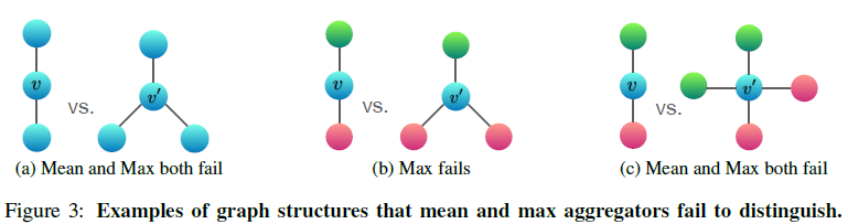
Figure 3 에서 node 의 색은 feature vector 를 의미합니다. 즉 같은 색을 가지면, 같은 feature vector 를 가집니다. 위에서 정의된 \(f\) 에 대해, \(f(red) > f(blue)>f(green)\) 을 만족한다고 가정하겠습니다. Figure 3-(a) 를 보면 non-isomorphic 한 두 그래프 모두 \(h_{max}\) 와 \(h_{mean}\) 의 결과가 \(f(blue)\) 로 같습니다. Figure 3-(c) 도 마찬가지로 non-isomorphic 한 두 그래프 모두 \(h_{max}=f(red)\), \(h_{mean}=\frac{1}{2}(f(red)+f(green))\) 으로 결과가 같습니다. Figure 3-(b) 의 경우 \(h_{mean}\) 은 값이 다르지만, \(h_{max}\) 의 값은 같습니다.

 

\((6)\) 에서는 다음과 같이 aggregator \(h\) 를 summation 으로 정의합니다.

\[h_{sum}\left( \left\{\!\!\left\{ h_u^{(k-1)} \,:\, u\in N(v) \right\}\!\!\right\} \right) = \sum_{u\in N(v)}f\left(h_u^{(k-1)}\right)\]

\(h_{sum}\) 이 multiset 전체를 injective 하게 표현할 수 있고, \(h_{mean}\) 의 경우 multiset 의 distribution 을, \(h_{max}\) 의 경우 multiset 의 서로다른 원소들로 이루어진 set 을 표현할 수 있다고 설명합니다.

 

따라서, max-pooling 과 mean-pooling 을 사용한 GraphSAGE 같은 경우 GIN 보다 representation power 가 떨어진다고 볼 수 있습니다.

 

Experiment & Result

 

논문에서는 GIN 과 다른 GNN 들의 graph classification 성능을 비교하기 위해, 4개의 bioinformatics datasets (MUTAG, PTC, NCI1, PROTEINS) 와 5개의 social network datasets (COLLAB, IMDB-BINARY, IMDB-MULTI, REDDIT-BINARY, REDDIT-MULTI5K) 에 대해 실험을 수행했습니다.

GIN 모델로 \((6)\) 에서 \(\epsilon\) 을 학습하는 GIN-\(\epsilon\) 과, \(\epsilon\) 을 0 으로 고정한 GIN-0 를 선택했습니다. GIN 과 비교하기 위해 \((6)\) 의 summation 을 \((9)\) 와 같이 mean-pooling 또는 max-pooling 으로 바꾸거나, MLP 를 1-layer perceptron 으로 바꾼 모델들 (Figure 4 의 Mean - 1-layer 와 같은 variant 들을 의미합니다.) 을 실험 대상으로 선정했습니다.

Baseline 모델로는 graph classification 의 state-of-the-art 성능을 보여주는 WL subtree kernel, C-SVM, Diffusion-convolutional neural network (DCNN), PATCHY-SAN, Deep Graph CNN (DGCNN), 그리고 Anonymous Walk Embeddings (AWL) 을 사용했습니다.

 

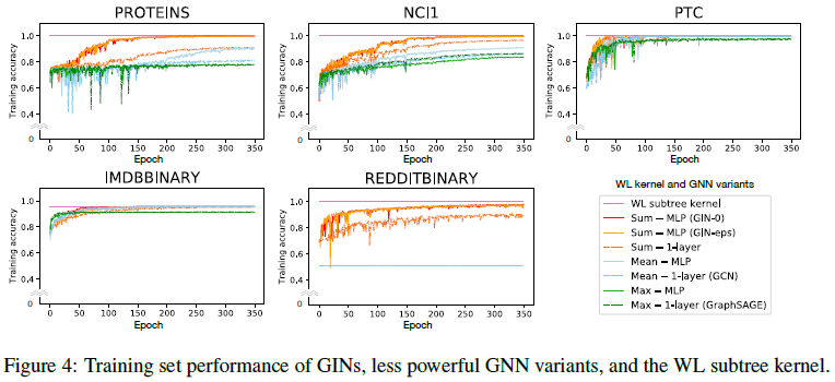
먼저 representational power 를 확인하기 위해 GNN 들의 training accuracy 들을 비교합니다. 모델의 representational power 가 높다면, training set 에서의 accuracy 또한 높아져야합니다. Figure 4 를 보면 GIN-\(\epsilon\) 과 GIN-0 모두 training accuracy 가 거의 1 에 수렴하는 것을 볼 수 있습니다. GIN-\(\epsilon\) 의 경우 각 layer 의 parameter \(\epsilon^{(k)}\) 또한 학습하지만, GIN-0 와 큰 차이를 보이지는 않습니다. Figure 4 에서 1-layer perceptron 보다는 MLP 를 사용했을 때, mean / max-pooling 보다는 summation 을 사용했을 때 정확도가 대체로 더 높게 나타납니다.

하지만 모든 GNN 모델들은 WL subtree kernel 의 정확도보다 낮은 것이 보입니다. Lemma 2 에서 설명했듯이, neighborhood aggregation scheme 을 사용하는 GNN 은 WL test 의 representational power 를 뛰어 넘을수 없다는 것을 확인할 수 있습니다.

 

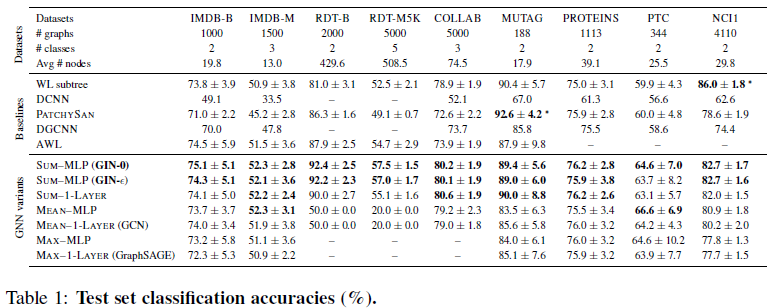
Table 1 은 test set 에 대한 classification accuracy 를 보여줍니다. GIN 모델, 특히 GIN-0 모델의 성능이 가장 뛰어나다는 것을 확인할 수 있습니다.

 

Reference

1. Xu, K., Hu, W., Leskovec, J., and Jegelka, S. (2019). How powerful are graph neural networks? In International Conference on Learning Representations.

2. Gilmer, J., Schoenholz, S. S., Riley, P. F., Vinyals, O., and Dahl, G. E. (2017). Neural message passing for quantum chemistry. In International Conference on Machine Learning, pages 1263–1272.

3. Zhengdao Chen, Soledad Villar, Lei Chen, and Joan Bruna. On the equivalence between graph isomorphism testing and function approximation with GNNs. In Advances in Neural Information Processing Systems, pages 15868–15876, 2019.

4. William L Hamilton, Rex Ying, and Jure Leskovec. Inductive representation learning on large graphs. In Advances in Neural Information Processing Systems (NIPS), pp. 1025–1035, 2017a.