Graph Convolution and Spectral Filtering

Graph Convolutional Network 이해하기 : (3) Graph convolution 과 spectral filtering

Why do we need Graph Convolution?

Fourier transform 을 통해 그래프에서 convolution 을 정의한 이유는, 바로 CNN 을 그래프에 적용하기 위해서입니다. CNN 은 ML 의 여러 분야에서 뛰어난 성과를 거두었습니다. 특히, CNN 은 large-scale high dimensional 데이터로부터 local structure 를 학습하여 의미있는 패턴을 잘 찾아냅니다. 이 때 local feature 들은 convolutional filter 로 표현되며, filter 는 translation-invariant 이기 때문에 공간적인 위치나 데이터의 크기에 상관없이 같은 feature 를 뽑아낼 수 있습니다.

하지만, 그래프와 같이 irregular (non-Euclidean) domain 에서는 직접 convolution 을 정의할 수 없습니다. 기존의 convolution 의 정의는 discrete 한 그래프에서는 의미를 갖지 못합니다. 따라서, Graph Convolutional Network 를 위해서는 그래프에서 정의되는 convolution operator 가 새로 필요합니다.

 

Graph Convolution

Vertex domain 에서 직접 convolution operator 를 정의할 수 없기 때문에, Fourier transform 을 이용하여 Fourier domain 에서 convolution operator 를 정의합니다.

기존의 convolution 과 같이 graph convolution 또한 Fourier transform 에 대해 다음의 조건을 만족해야 합니다. (Convolution theorem).

\[\widehat{g\ast f}(l) = \hat{g}(l)\hat{f}(l) \tag{1}\]

즉 vertex domain 에서의 convolution 과 Fourier domain 에서의 multiplication 이 일치하도록 만들고 싶습니다. \((1)\) 에 대해 inverse Fourier transform 을 적용하면, 다음의 결과를 얻게 됩니다.

\[g\ast f = \sum^{N-1}_{l=0} \hat{g}(l) \hat{f}(l)u_l \tag{2}\]

따라서, vertex domain 에서 정의된 두 graph signal \(f\) 와 \(g\) 에 대해 convolution operator \(\ast\) 는 \((2)\) 과 같이 정의합니다. 이는 기존의 convolution 에서 complex exponential \(\left\{e^{2\pi i\xi t}\right\}_{\xi\in\mathbb{R}}\) 대신 graph Laplacian eigenvector \(\{u_l\}^{N-1}_{l=0}\) 을 사용했다고 이해할 수 있습니다. \((2)\) 는 Hadamard product \(\odot\) 와 \(\{u_l\}^{N-1}_{l=0}\) 을 column vector 로 가지는 Fourier basis \(U\) 를 사용해, 다음과 같은 형태로 표현할 수 있습니다.

\[g \ast f = U((U^Tg) \odot (U^Tf)) \tag{3}\]

 

Spectral Filtering of Graph Signal

위에서 정의한 graph convolution 을 사용해, 다음과 같이 graph signal \(f_{in}\) 의 \(g\) 에 대한 filtering 을 정의할 수 있습니다.

\[f_{out} = g\ast f_{in}\]

\((1)\) 을 사용하면 filtering 은 다음과 같이 표현할 수 있습니다.

\[\begin{align} f_{out} &= \sum^{N-1}_{l=0} \hat{f}_{out}(l)u_l \\ &= \begin{bmatrix} \big| & \big| & & \big| \\ u_0 & u_1 & \cdots & u_{N-1} \\ \big| & \big| & & \big| \end{bmatrix} \begin{bmatrix} \hat{f}_{out}(0) \\ \vdots \\ \hat{f}_{out}({N-1}) \end{bmatrix} \\ \\ &= U \begin{bmatrix} \hat{g}(0)\hat{f}_{in}(0) \\ \vdots \\ \hat{g}({N-1})\hat{f}_{in}({N-1}) \end{bmatrix} \\ \\ &= U \begin{bmatrix} \hat{g}(0) & 0 & \cdots & 0 \\ 0 & \hat{g}(1) & \cdots & 0 \\ \vdots & & \ddots & \\ 0 & 0 & 0 & \hat{g}({N-1}) \end{bmatrix} \begin{bmatrix} \hat{f}_{in}(0) \\ \vdots \\ \hat{f}_{in}({N-1}) \end{bmatrix} \\ \\ &= U\,\text{diag}(\hat{g})\,U^T f_{in} \tag{4} \end{align}\]

\((4)\) 를 통해 convolution operator 는 Fourier domain 에서 diagonalize 되는 operator 로 이해할 수 있습니다.

Reference 의 [1, 2] 에서는 \(\text{diag}(\hat{g})\) 를 함수가 아닌, filter 의 parameter 로 해석했습니다. 이를 spectral construction 이라 부르며, vertex domain 에서 localized filter 를 사용하는spatial construction 에 비해 parameter 의 수를 \(N^2\) 에서 \(N\) 으로 줄였다는데 의의가 있습니다. 하지만, Fourier basis \(U\) 를 사용하기 위해서는 computational cost 가 높은 eigenvalue decomposition 을 수행해야 하기 때문에, 효율적인 방법이 아닙니다.

이런 문제를 해결하기 위해 [3] 에서는 \(g_{\theta}\) 로 \(L\) 의 eigenvalue 들에 대한 polynomial 을 사용했습니다. 이 경우, \(L = U\Lambda U^T\) 를 만족하기 때문에, \(U\) 대신 \(L\) 로써 \((5)\) 를 표현할 수 있고, eigen decomposition 을 하지 않아도 되기 때문에 굉장히 효율적입니다.

따라서 GCN 에서의 spectral convolution 은 \(\hat{g}\) 을 \(L\) 의 eigenvalue 에 대한 함수 \(g_{\theta}\) 로 생각하고, \(\text{diag}(\hat{g})\) 대신 다음의 \(g_\theta(\Lambda)\) 를 사용하여 \((4)\) 를 표현합니다.

\[g_{\theta}(\Lambda) = \begin{bmatrix} g_{\theta}(\lambda_0) & 0 & \cdots & 0 \\ 0 & g_{\theta}(\lambda_1) & \cdots & 0 \\ \vdots & & \ddots & \\ 0 & 0 & 0 & g_{\theta}(\lambda_{N-1}) \end{bmatrix}\]

따라서, \(g_{\theta}\) 에 대한 filtering 의 결과는 다음과 같습니다.

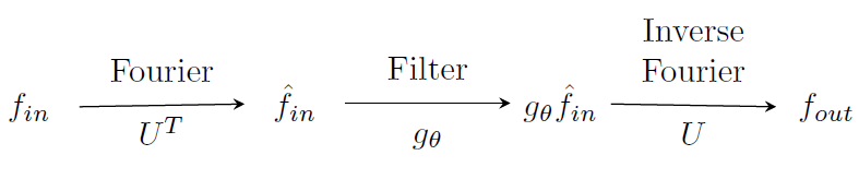
\[f_{out} = Ug_{\theta}(\Lambda)U^T f_{in} \tag{5}\]

\((5)\) 의 spectral filtering 은 다음과 같이 Fourier domain 에서 \(g_{\theta}\) 에 대한 filtering 으로 이해할 수 있습니다.

 

Reference

1. Joan Bruna, Wojciech Zaremba, Arthur Szlam, and Yann LeCun. Spectral networks and locally connected networks on graphs. In International Conference on Learning Representations (ICLR), 2014.

2. M. Henaff, J. Bruna, and Y. LeCun. Deep Convolutional Networks on Graph-Structured Data. arXiv:1506.05163, 2015.

3. Michael Defferrard, Xavier Bresson, and Pierre Vandergheynst. Convolutional neural networks on graphs with fast localized spectral filtering. In Advances in neural information processing systems (NIPS), 2016.

4. Thomas N. Kipf and Max Welling. Semi-supervised classification with graph convolutional networks. In International Conference on Learning Representations (ICLR), 2017.

5. David K Hammond, Pierre Vandergheynst, and Remi Gribonval. Wavelets on graphs via spectral graph theory. Applied and Computational Harmonic Analysis, 30(2):129–150, 2011.