Graph Fourier Transform

Graph Convolutional Network 이해하기 : (2) Graph Fourier transform

Classical Fourier Transform

Fourier transform

Integrable function \(f : \mathbb{R} \rightarrow \mathbb{C}\) 의 Fourier transform 은 다음과 같이 정의합니다.

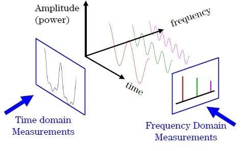
\[\hat{f}(\xi) = \langle f, e^{2\pi i\xi t} \rangle = \int_{\mathbb{R}} f(t) e^{-2\pi i\xi t}dt \tag{$1$}\]

즉 \(\hat{f}(\xi)\) 은 \(f(t)\) 의 \(e^{2\pi i \xi t}\) 성분 (frequency) 의 크기 (amplitude) 를 의미합니다. \((1)\) 을 살펴보면, Fourier transform 은 time domain \(t\in\mathbb{R}\) 에서 정의된 함수 \(f(t)\) 를 frequency domain \(\xi\in\mathbb{C}\) 에서 정의된 함수 \(\hat{f}(\xi)\) 로 변환시켜준다는 것을 알 수 있습니다. 다음의 그림을 통해 time domain 으로부터 frequency domain 으로의 Fourier transform 을 이해할 수 있습니다.

Inverse Fourier transform

\((1)\) 에서 정의된 Fourier transform 의 역과정인 inverse Fourier transform 은 다음과 같습니다.

\[f(x) = \int_{\mathbb{R}} \hat{f}(\xi)e^{2\pi i\xi t}d\xi \tag{$2$}\]

Invere Fourier transform 은 Fourier transform 과 반대로 frequency domain 에서 정의된 함수 \(\hat{f}\) 을 time domain 에서의 함수 \(f\) 로 변환시켜줍니다. \((2)\) 는 주어진 \(\hat{f}\) 으로부터 원래의 함수 \(f\) 를 복원하는 과정이며, 각 \(e^{2\pi i \xi t}\) 성분의 amplitude \(\hat{f}(\xi)\) 이 주어졌을 때 원래의 함수 \(f\) 를 각 성분들의 합으로 표현하는 변환입니다.

Laplacian operator

\((1)\) 과 \((2)\) 에서 등장하는 complex exponentials \(\left\{ e^{2\pi i \xi t} \right\}_{\xi\in\mathbb{C}}\) 는 1 차원 Laplacian operator \(\Delta\) 의 eigenfunction 입니다.

\[\Delta(e^{2\pi i \xi t}) = \frac{\partial^2}{\partial t^2}e^{2\pi i \xi t} = -(2\pi\xi)^2 e^{2\pi i \xi t}\]

즉 Fourier transform 은 Laplacian operator \(\Delta\) 의 eigenfunction 들의 합으로 분해하는 변환으로 생각 할 수 있습니다. [3]

 

Graph Fourier Transform

Graph Fourier transform

그래프에서의 graph Laplacian \(L\) 은 Euclidean space 의 Laplacian operator \(\Delta\) 와 같은 역할을 합니다. 특히, 1 차원 Laplacian operator \(\Delta\) 에 대해 complex exponential 들은 eigenfunction 이며, 그래프에서는 \(L\) 의 eigenvector 들이 그 역할을 대신합니다.

이 때 graph Laplacian 의 eigenvector 들로 \(\mathbb{R}^N\) 의 orthonormal basis 를 구성할 수 있기 때문에, orthonormal eigenvector \(\left\{ u_l \right\}^{N-1}_{l=0}\) 을 사용해 \((2)\) 와 같이 graph Fourier transform 을 정의할 수 있습니다. Euclidean space 에서 compex exponential 들이 Fourier basis 를 이루듯이, 그래프에서는 eigenvector \(\left\{ u_l \right\}^{N-1}_{l=0}\) 들이 Fourier basis 가 됩니다.

Graph signal \(f \in\mathbb{R}^{N}\) 에 대한 Fourier transform 은 \(\left\{ u_l \right\}^{N-1}_{l=0}\) 성분들의 합으로 분해하는 변환으로 이해할 수 있습니다. \(u_l\) 성분의 크기 (amplitude) 는 inner product 를 사용해 다음과 같이 계산할 수 있습니다.

\[\hat{f}(l) = \langle u_l, f\rangle = \sum^N_{i=1} u^{T}_l(i)f(i) \tag{3}\]

\(\hat{f}\) 을 다음과 같이 \(\mathbb{R}^N\) 의 vector 로 생각하겠습니다.

\[\hat{f} = \begin{bmatrix} \hat{f}(0) \\ \vdots \\ \hat{f}({N-1}) \end{bmatrix}\]

\(L\) 의 eigenvector \(\left\{ u_l \right\}^{N-1}_{l=0}\) 를 column 으로 가지는 행렬 \(U\) 에 대해

\[U = \begin{bmatrix} \bigg| & \bigg| & & \bigg| \\ u_0 & u_1 & \cdots & u_{N-1} \\ \bigg| & \bigg| & & \bigg| \end{bmatrix}\]

\((3)\) 를 다음과 같이 표현할 수 있습니다.

\[\hat{f} = \begin{bmatrix} \hat{f}(0) \\ \vdots \\ \hat{f}({N-1}) \end{bmatrix} = \begin{bmatrix} - & u_0^{T} & - \\ & \vdots & \\ - & u_{N-1}^{T} & - \end{bmatrix} \begin{bmatrix} f(1) \\ \vdots \\ f(N) \end{bmatrix} = U^{T}f\]

따라서, graph signal \(f\) 에 대한 graph Fourier transform 은 Fourier basis \(U\) 를 사용해 다음과 같이 쓸 수 있습니다. \(\hat{f} = U^T f \tag{4}\)

 

Inverse graph Fourier transform

Inverse Fourier transform 과 마찬가지로, inverse graph Fourier transform 은 graph Fourier transform 의 역과정입니다. 그렇기 때문에, \((5)\) 에서 정의된 graph Fourier transform 을 되돌리는 과정은 다음과 같습니다.

\[f \overset{\mathrm{(a)}}{=} UU^Tf = U\hat{f} \tag{5}\]

위의 식에서 Fourier basis 가 orthonormal 하기 때문에 \(UU^T = I\) 이므로 \((a)\) 가 성립합니다.

\((6)\) 의 결과는 \(\hat{f}\) 의 의미를 통해서 유도할 수 있습니다. \(\left\{ u_l \right\}^{N-1}_{l=0}\) 은 \(\mathbb{R}^N\) 의 orthonormal basis 를 이루기 때문에, Fourier transform 의 결과인 \(\hat{f}\) 으로 부터 원래의 \(f\) 를 얻어내기 위해서는 각 성분들을 모두 더해주면 됩니다. 이 때, \(f\) 의 \(u_l\) 성분의 크기는 \(\hat{f}(l)\) 이기 때문에, 다음의 등식이 성립합니다.

\[f(i) = \sum^{N-1}_{l=0} \hat{f}(l)u_l(i) \tag{6}\]

\((6)\) 를 \(\mathbb{R}^N\) 의 vector 로 표현하면, \((5)\) 의 결과와 일치합니다.

\[f = \begin{bmatrix} f(1) \\ \vdots \\ f(N) \end{bmatrix} = \begin{bmatrix} \bigg| & \bigg| & & \bigg| \\ u_0 & u_1 & \cdots & u_{N-1} \\ \bigg| & \bigg| & & \bigg| \end{bmatrix} \begin{bmatrix} \hat{f}(0) \\ \vdots \\ \hat{f}({N-1}) \end{bmatrix} = U\hat{f}\]

Parseval relation

Classical Fourier transform 에서와 마찬가지로, graph Fourier transform 은 Parseval relation 을 만족합니다.

\[\begin{align} \langle f, g\rangle &= \langle \sum^{N-1}_{l=0}\hat{f}(l)u_l, \sum^{N-1}_{l'=0}\hat{g}({l'})u_{l'} \rangle \\ &= \sum_{l, l'} \hat{f}(l)\hat{g}({l'})\langle u_l, u_{l'} \rangle \\ &= \sum_{l} \hat{f}(l)\hat{g}(l) = \langle \hat{f}, \hat{g} \rangle \end{align}\]

 

Reference

1. David K. Hammond, Pierre Vandergheynst, and Remi Gribonval. Wavelets on graphs via spectral graph theory. Applied and Computational Harmonic Analysis, 30(2):129–150, 2011.

2. Michael Defferrard, Xavier Bresson, and Pierre Vandergheynst. Convolutional neural networks on graphs with fast localized spectral filtering. In Advances in neural information processing systems (NIPS), 2016.

3. Terence Tao, Fourier Trasnform