Graph Laplacian

Graph Convolutional Network 이해하기 : (1) Graph Laplacian

Basic definition

Weighted adjacency Matrix

주어진 undirected weighted graph \(G = (V,E,W)\) 는 vertices 의 집합 \(V\), edges 의 집합 \(E\), 그리고 weighted adjacency matrix \(W\) 로 이루어집니다. 이 포스트에서는 \(\vert V\vert= N < \infty\) 을 가정합니다. 편의상 \(V = \{1,2,\cdots,N\}\) 으로 나타내겠습니다. 여기서 vertices 의 ordering 은 임의로 주어진 것이며, 의미를 가지지 않습니다.

\(E\) 의 원소 \(e = (i,j)\) 는 vertex \(i\) 와 \(j\) 를 연결하는 edge 를 나타냅니다. 또한 \(W_{ij}\) 는 edge \(e = (i,j)\) 의 weight 을 의미하며 만약 \(i\) 와 \(j\)를 연결하는 edge 가 없다면 \(W_{ij}=0\) 이고 edge 가 있는 경우 \(W_{ij}>0\) 입니다. 이 때 \(W\) 는 모든 vertex pair 마다 정의되고 그래프가 undirected 이므로, \(W\) 는 \(N\times N\) real symmetric matrix 입니다.

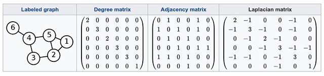
Weighted adjacency matrix 의 한 예로 adjacency matrix 가 있습니다. Adjacency matrix 는 \(i\) 와 \(j\) 를 연결하는 edge 가 있다면 \(W_{ij} = 1\), 없다면 \(W_{ij}=0\) 으로 정의합니다. 다음의 그림은 그래프 (labeled) 에 대한 adjacency matrix 의 예시입니다.

Degree matrix

주어진 weighted adjacency matrix \(W\) 에 대해 degree matrix \(D\) 는 다음을 만족하는 diagonal matrix 로 정의합니다. \(D_{ii} = \sum^{N}_{j=1} W_{ij} \tag{1}\)

쉽게 말해, \(D_{ii}\) 는 vertex \(i\) 를 끝점으로 가지는 edge 들의 weight 를 모두 더한 값과 같습니다. 특히 adjacency matrix 에 대해서는 \((1)\) 의 합이 각 vertex 의 degree 를 의미하기 때문에 degree matrix 라는 명칭이 붙었습니다.

 

Unnormalized Graph Laplacian

주어진 undirected weighted graph \(G = (V,E,W)\) 에 대해 unnormalized graph Laplacian 은 다음과 같이 정의됩니다.

\[L = D-W\]

여기서 \(D\) 는 앞서 정의한 degree matrix 입니다. Unnormalized graph Laplacain 은 combinatorial Laplacian 이라고도 불립니다.

다음은 예시 그래프에 대한 adjacency matrix, degree matrix, 그리고 graph Laplacian matrix 를 보여줍니다.

Unnormalized graph Laplacian 은 다음과 같은 특징을 가집니다.

Real symmetric

Undirected weighted graph \(G\) 에 대해 \(W\) 와 \(D\) 는 \(N\times N\) real symmetric matrix 이므로, \(L=D-W\) 또한 \(N\times N\) real symmetric matrix 입니다.

Positive semi-definite

임의의 \(x\in\mathbb{R}^N\) 에 대해,

\[\begin{align} x^TLx &= x^TDx - x^TWx = \sum_{i} D_{ii}x_i^2 - \sum_{i,j}x_iW_{ij}x_j \\ &= \frac{1}{2} \left( 2\sum_{i} D_{ii}x_i^2 - 2\sum_{i,j} W_{ij}x_ix_j \right) \\ &\overset{\mathrm{(a)}}{=} \frac{1}{2}\left( 2\sum_{i}\left\{\sum_{j}W_{ij}\right\} x_i^2 - 2\sum_{i,j} W_{ij}x_ix_j \right) \\ &\overset{\mathrm{(b)}}{=} \frac{1}{2}\left( \sum_{i,j}W_{ij}x_i^2 + \sum_{i,j}W_{ij}x_j^2 - 2\sum_{i,j} W_{ij}x_ix_j \right) \\ &= \frac{1}{2}\sum_{i,j} W_{ij}(x_i-x_j)^2 \geq 0 \tag{2} \end{align}\]

유도 과정에서 \((a)\) 는 degree matrix 의 정의를 사용하였고, \((b)\) 는 \(W\) 가 symmetric 이기 때문에 성립합니다. 따라서 \(L\) 은 positive semi-definite matrix 입니다.

Non-negative eigenvalue

\(L\) 이 positive semi-definite matrix 이므로, \(L\) 은 non-negative real eigenvalue 들을 가집니다.

Orthonormal basis

\(L\) 은 real symmetric matrix 이기 때문에 다음의 lemma 를 이용하면, \(L\) 의 eigenvector 들로 \(\mathbb{R}^N\) 의 orthonormal basis 를 만들 수 있습니다.

__Lemma : __ Real symmetric matrix 는 diagonalizable 합니다.

Multiplicity of zero

\(u_0 = \frac{1}{\sqrt{N}}\begin{bmatrix} 1 & 1 & \cdots & 1 \end{bmatrix}^T\) 에 대해 다음을 만족하기 때문에,

\[Lu_0 = (D-W)u_0 = \mathbf{0}\]

\(L\) 은 0 을 eigenvalue 로 가지며 \(u_0\) 는 \(L\) 의 eigenvector 입니다. 이 때, 주어진 그래프와 상관 없이 \(L\) 은 항상 0 을 eigenvalue 로 가지고 \(u_0 = \frac{1}{\sqrt{N}}\begin{bmatrix} 1 & 1 & \cdots & 1 \end{bmatrix}^T\) 또한 항상 eigenvector 가 됩니다.

0 의 eigenvector \(u\) 에 대해 \((2)\) 의 결과를 이용하면, 다음과 같습니다. \(0 = u^TLu = \frac{1}{2}\sum_{i,j}W_{ij}(u(i) - u(j))^2\)

따라서 \(W_{ij}\neq 0\) 인 모든 vertices \(i\) 와 \(j\) , 즉 edge로 연결된 \(i\) 와 \(j\) 에 대해 \(u(i) = u(j)\) 를 만족합니다. \((\ast)\)

\(k\) 개의 connected components 를 가지는 그래프 \(G\) 의 graph Laplacian \(L\) 은

\[L = \begin{bmatrix} L_1 & & & \\ & L_2 & & \\ & & \ddots & \\ & & & L_k \end{bmatrix}\]

sub-Laplacian \(L_i\) 들로 이루어진 block matrix 로 볼 수 있습니다.

각각의 sub-Laplacian 들은 모두 0 을 eigenvalue 로 가지고, eigenvector \(u\) 는 \((\ast)\) 로 인해 \(u_0\) 로 유일하게 결정되기 때문에 각각의 sub-Laplacian 들은 정확히 한 개의 eigenvalue 0 을 가집니다. \(k\) 개의 connected components 를 가지는 그래프에 대해서 \(L\) 은 정확히 \(k\) 개의 eigenvalue 0 들을 가집니다. 따라서 graph Laplacian \(L\) 의 eigenvalue 0 의 multiplicity 는 주어진 그래프 \(G\) 의 connected components 의 개수와 일치합니다 [3].

 

주어진 그래프를 connected 라고 가정하면 \(L\) 의 eigenvalue 들을 다음과 같이 나열할 수 있습니다.

\[0 = \lambda_0 < \lambda_1 \leq \cdots \leq \lambda_{N-1}\]

\(L\) 의 eigenvalue 들, 즉 spectrum 을 다루는 분야가 바로 spectral graph theory 입니다. Spectral graph theory 에 포함된 Fideler vector, Cheegar Constant, Laplacian embedding, NCut 등에 대해서는, 기회가 생기면 다른 포스트를 통해 자세히 설명하겠습니다.

 

Other Graph Laplacians

Normalized graph Laplacian

Normalized graph Laplacian \(L^{norm}\) 은 다음과 같이 정의합니다.

\[L^{norm} = D^{-1/2}\;L\;D^{-1/2} = I - D^{-1/2}\;W\;D^{-1/2}\]

\(L\) 과 같이 symmetric positive semi-definite matrix 입니다. 따라서 위에서 설명한 eigenvalue 에 대한 성질이 동일하게 적용됩니다. 하지만 \(L\) 과 \(L^{norm}\) 은 similar matrices 가 아니기 때문에 다른 eigenvector 를 가집니다. 특히 \(L\) 의 eigenvalue 0 에 대한 eigenvector \(u_0\) 는 그래프에 상관 없이 일정하지만, \(L^{norm}\) 의 경우 그래프에 따라 변합니다. Normalized graph Laplacian 의 특징으로는, eigenvalue 들이 \([0,2]\) 구간에 속한다는 것입니다. 그래프 \(G\) 가 bipartite graph 일 때만 \(L^{norm}\) 의 가장 큰 eigenvalue 가 2가 됩니다 [3].

Random walk graph Laplacian

Random walk graph Laplacian \(L^{rw}\) 는 다음과 같이 정의합니다.

\[L^{rw} = D^{-1}L = I - D^{-1}W\]

여기서 \(D^{-1}W\) 는 random walk matrix 로 그래프 \(G\) 에서의 Markov random walk 를 나타내어 줍니다. \(L^{rw}\) 는 symmetric 이 보장되지 않습니다.

 

Reference

1. D. Shuman, S. Narang, P. Frossard, A. Ortega, and P. Vandergheynst. The Emerging Field of Signal Processing on Graphs: Extending High-Dimensional Data Analysis to Networks and other Irregular Domains. IEEE Signal Processing Magazine, 30(3):83–98, 2013.

2. David K Hammond, Pierre Vandergheynst, and Remi Gribonval. Wavelets on graphs via spectral graph theory. Applied and Computational Harmonic Analysis, 30(2):129–150, 2011.

3. F. R. K. Chung. Spectral Graph Theory, volume 92. American Mathematical Society, 1997.